Langer LFS Scanner Probes | 100 kHz to 50 MHz
100 kHz to 50 MHz | 1 probe models | Passive | SMA connection
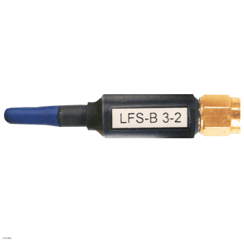
LFS-B 3 is a passive H-field scanner probe for low-frequency magnetic-field investigations. Its orthogonal coil and perpendicular approach help reach PCB structures between taller components.
MARKETS:
CATEGORIES:
TEST STANDARDS:
Select Options/Sizes:

LFS-B 3 - Datasheet
SPECIFICATIONS
LFS scanner probes
LFS-B 3 is a passive H-field scanner probe for low-frequency magnetic-field investigations. Its orthogonal coil and perpendicular approach help reach PCB structures between taller components.
All published scalar specifications are consolidated below. Click each small response, correction-curve or geometry image to open the full-size image in a new tab. Missing numeric resolution or length values are not inferred from model names or photographs.
| Specification / view | LFS-B 3 |
|---|---|
| Product picture |  |
| Field type | H-field |
| Frequency range | 100 kHz ... 50 MHz |
| Resolution | approx. 2 mm |
| Probe head dimensions | diameter approx. 4 mm |
| Connector - output | SMA, male, jack |
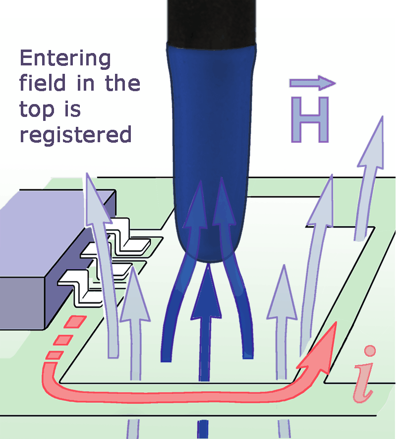
| Use and orientation | H-field; coil orthogonal to the shaft. Place the shaft perpendicular to the board for access between taller components; suited to low-frequency switching-current investigations. |
| Sensing orientation Click image for full view |
 Sensing orientation / measuring principle |
| Additional views Click image for full view |
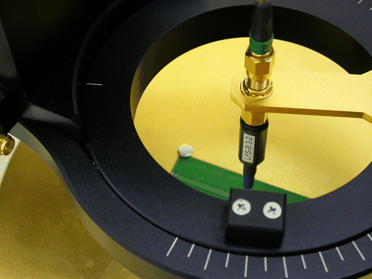
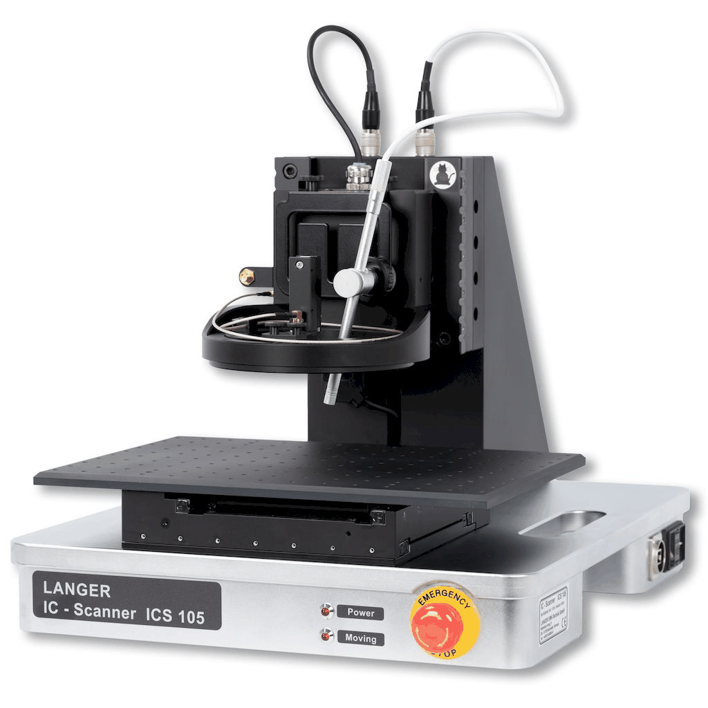
 LFS-B 3-2 scanner probe connected to ICS 105 scanner |
| Frequency response Click image for full view |
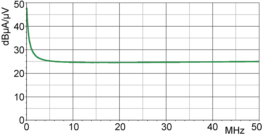
 Frequency response [dBuV] / [dBuA/m] |
| H-field correction curve Click image for full view |
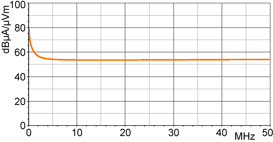
 H-field correction curve [dBuA/m] / [dBuV] |
| Current correction curve Click image for full view |
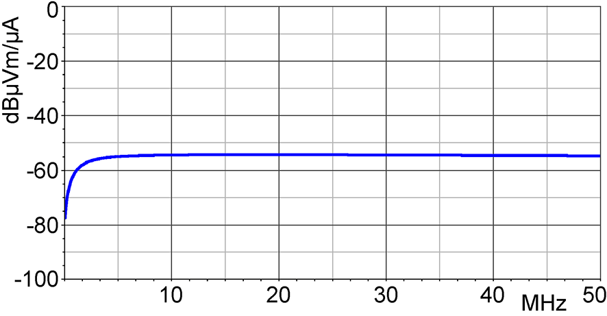
 Current correction curve [dBuA] / [dBuV] |
Using the curves and geometries
Frequency-response plots show the model-specific response. H-field, E-field and current correction curves are separate quantities: use the appropriate curve, units, distance and setup when converting receiver voltage to a field or current estimate. A probe is directional; keep the sensing orientation and probe-to-DUT spacing consistent between scans. The source tables use both "SMA male plug" and "SMA male jack" wording; verify the mating cable rather than silently treating the terms as different probe genders.
Datasheets and reference documents
| Product | Document |
|---|---|
| LFS-B 3 | LFS-B 3 - Datasheet |
Scanner probe family comparison
| Family | Models | Coverage | Field types | Choose for |
|---|---|---|---|---|
| LFS |
1 | 100 kHz-50 MHz | H | Low-frequency switching-current and magnetic-field mapping. |
 RFS |
7 | 30 MHz-3 GHz | H and E | General PCB investigations with large-area and fine-resolution geometries. |
 XFS |
4 | 30 MHz-6 GHz | H and E | PCB near-field mapping when coverage above 3 GHz is needed. |
The passive scanner probes below have model-specific SMA connections and no power supply in their published specification. ICR near-field microprobes are a separate precision-probe class; use the existing ICR near-field microprobe range when micrometer-scale sensing is needed.
OTHER PRODUCTS IN THE SAME CATEGORY:
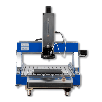
Langer FLS 106 IC | Large-area scanner with probe rotation
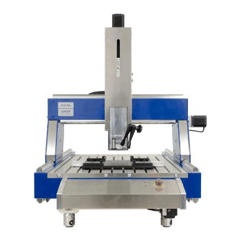
Langer FLS 106 PCB | Large-area three-axis PCB scanner
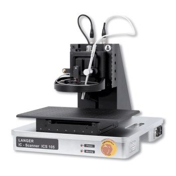
Langer Scanner and Scanner Probe Comparison Guide
Langer LFS Scanner Probes | 100 kHz to 50 MHz
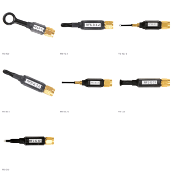
Langer RFS Scanner Probes | 30 MHz to 3 GHz
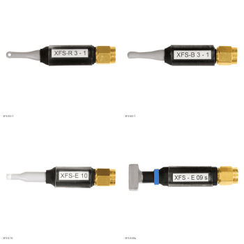
Langer XFS Scanner Probes | 30 MHz to 6 GHz
EMProbe CR5 - Custom Large-Reach Robotic EMI Scanning System
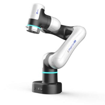
EMProbe-DBM-E6 — 6-Axis Robotic Near-Field EMI Diagnostics on the Bench
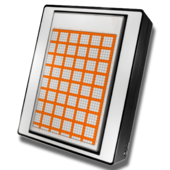
EMScanner+: 150 kHz- 6 GHz, w/ Real-Time Spectrum Analyzer, EMC desktop scanner
EMScannerR+: 150 kHz- 6 GHz, w/ Real-Time Spectrum Analyzer, EMC desktop scanner
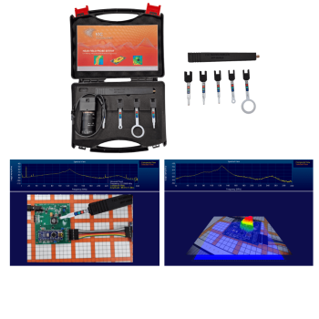
NFPKIT, EM Near Field Probe Kit w/Camera & Software
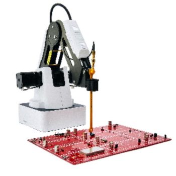
EMProbe: 9kHz- 18 GHz, 0.2mm resolution, EMC robotic scanner
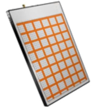
EMScanner: 150 kHz- 8 GHz, 3.5mm Resolution, EMC desktop scanner
EMScannerR: 150 kHz- 8 GHz, 0.06mm resolution, EMC desktop scanner
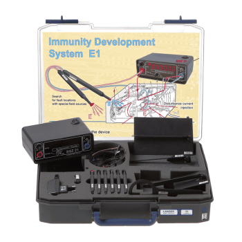
Langer E1 set | PCB Immunity Development System
Langer Scanner and Scanner Probe Comparison Guide
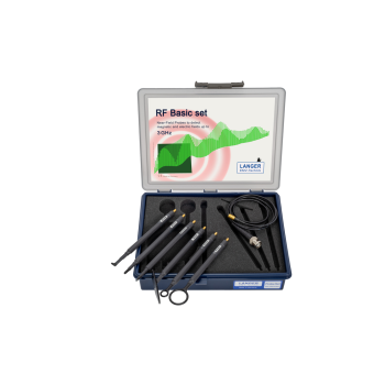
Langer Handheld Near-Field Probes Selection Guide
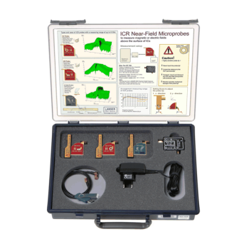
Langer ICR Near-Field Microprobe Selection Guide
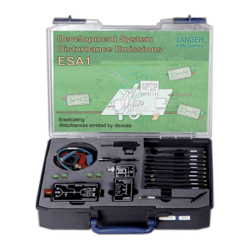
Langer ESA1 Set | EMC Emission Development System