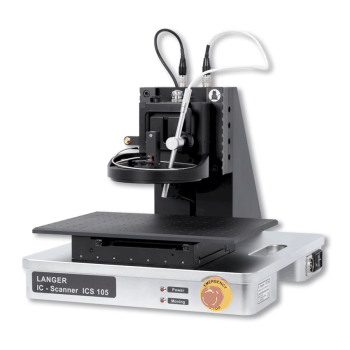
Langer Scanner and Scanner Probe Comparison Guide
3 scanner platforms | Full and Basic packages | 12 passive scanner probes
Compare travel, axes, minimum step, speed, footprint, field type, probe geometry and frequency range before configuring an EMC scanning system.
MARKETS:
CATEGORIES:
TEST STANDARDS:

Spectrum Analyzer Compatibility
SPECIFICATIONS
Select a scanner by DUT size, rotation and workflow
Choose the motion platform for the DUT footprint and required axes, then select a probe by frequency, field type, geometry and spatial scale. A finer motion step does not make a large probe resolve a smaller field source.
Scanner comparison - differences that matter
| Scanner | Best fit / benefit | Travel and axes | Minimum step | Positioning speed | Weight / footprint |
|---|---|---|---|---|---|
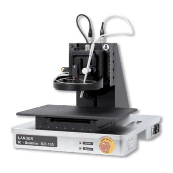 ICS 105 |
Compact IC workbench scanner Choose for a small IC scan area, finer minimum positioning increment and a compact bench footprint. |
50 x 50 x 50 mm; +/-180 deg | 10 um linear; 1 deg rotation | 10 / 10 / 5 mm/s; 90 deg/s | 23 kg; 350 x 400 x 420 mm |
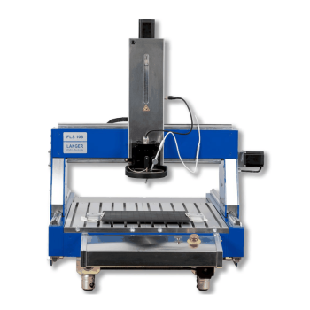 FLS 106 IC |
Large-area scanner with probe rotation Choose when the DUT or fixture needs a larger area and IC-style angular probe scans are important. |
400 x 600 x 120 mm; +/-180 deg | 20 um linear; 1 deg rotation | 20 / 25 / 10 mm/s; 90 deg/s | 75 kg; 1030 x 775 x 900 mm |
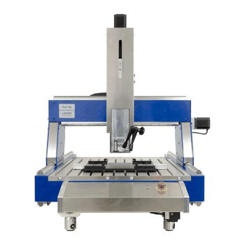 FLS 106 PCB |
Large-area three-axis PCB scanner Choose for repeatable X/Y/Z scans over assemblies without the IC model's motorized alpha rotation. |
400 x 600 x 120 mm; no alpha axis | 20 um linear | 20 / 25 / 10 mm/s | 75 kg; 1030 x 775 x 900 mm |
Travel, step size and speed are listed in X/Y/Z order. Minimum positioning step is not probe spatial resolution, repeatability or positioning accuracy. Achievable field-map detail depends on probe size, spacing, orientation and the complete measurement chain. Scanner frequency coverage is determined by the selected probe and RF instrument, not the motion platform.
Full set or Basic?
| Package | Choose when | Software / accessories |
|---|---|---|
| Full set | You want ChipScan-Scanner acquisition and analysis without building your own control workflow. | Software license included. Read each model's exact delivery table. |
| Basic set | You plan to integrate the scanner into an existing or custom automation environment. | ChipScan-Scanner not included; SDK/API and receiver integration must be configured. Some accessory contents differ. |
Scanner probe family comparison
| Family | Models | Coverage | Field types | Choose for |
|---|---|---|---|---|
 LFS |
1 | 100 kHz-50 MHz | H | Low-frequency switching-current and magnetic-field mapping. |
 RFS |
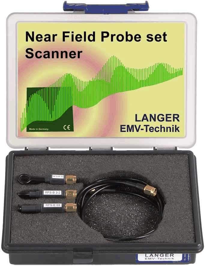
7 | 30 MHz-3 GHz | H and E | General PCB investigations with large-area and fine-resolution geometries. |
 XFS |
4 | 30 MHz-6 GHz | H and E | PCB near-field mapping when coverage above 3 GHz is needed. |
The passive scanner probes below have model-specific SMA connections and no power supply in their published specification. ICR near-field microprobes are a separate precision-probe class; use the existing ICR near-field microprobe range when micrometer-scale sensing is needed.
Compare every LFS, RFS and XFS scanner probe
LFS probe specifications
| Specification / view | LFS-B 3 |
|---|---|
| Product picture | |
| Field type | H-field |
| Frequency range | 100 kHz ... 50 MHz |
| Resolution | approx. 2 mm |
| Probe head dimensions | diameter approx. 4 mm |
| Connector - output | SMA, male, jack |
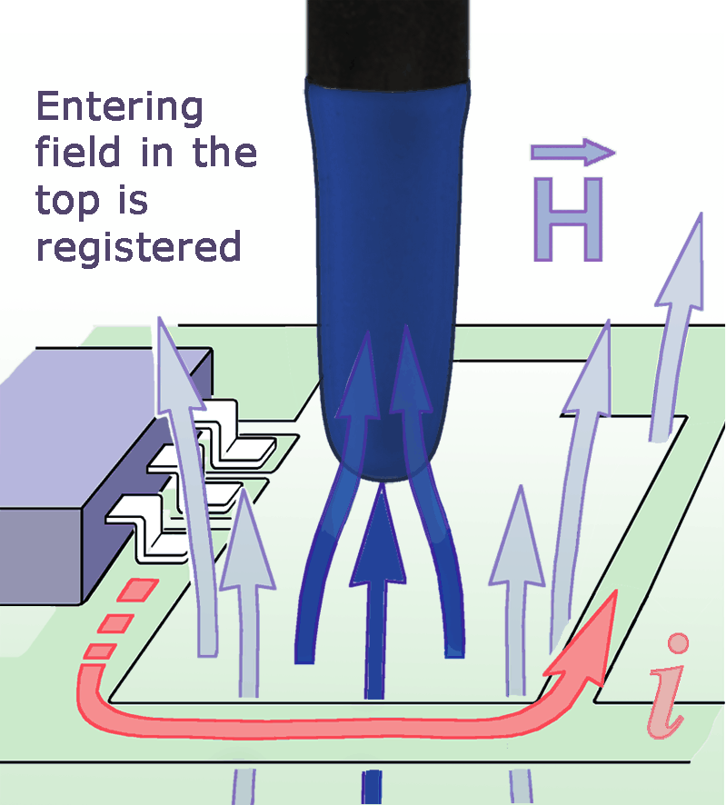
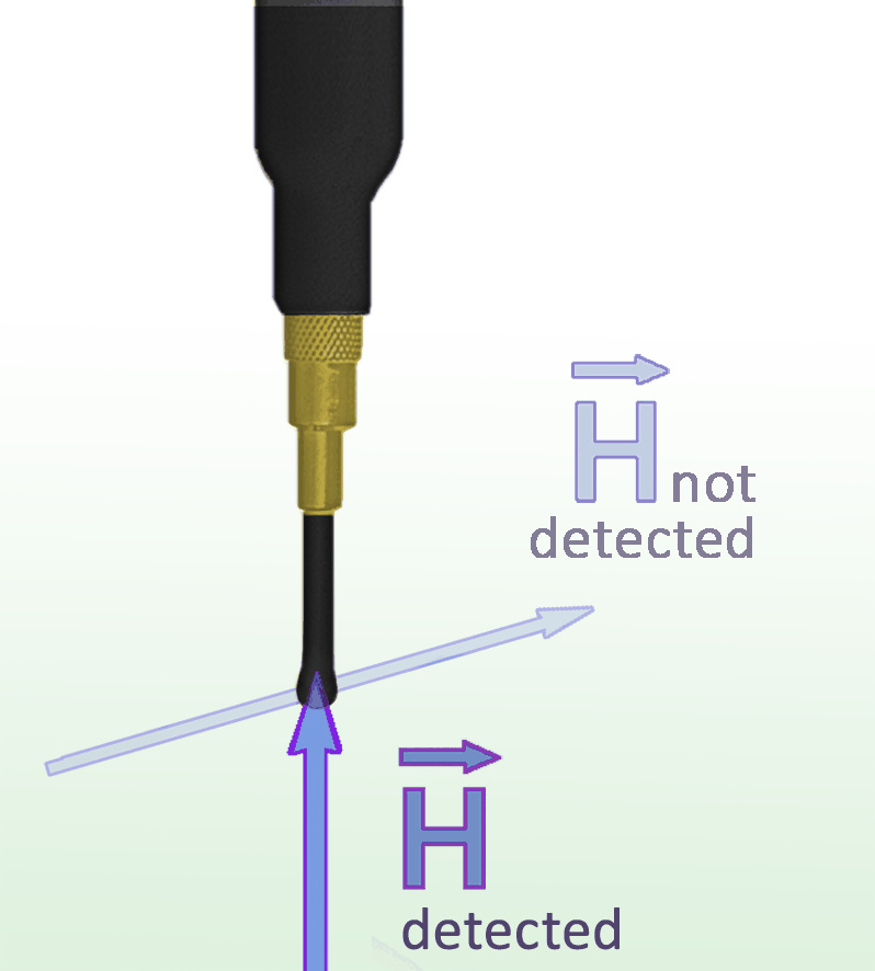
| Use and orientation | H-field; coil orthogonal to the shaft. Place the shaft perpendicular to the board for access between taller components; suited to low-frequency switching-current investigations. |
| Sensing orientation Click image for full view |
 Sensing orientation / measuring principle |
| Additional views Click image for full view |
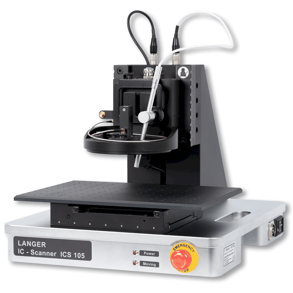
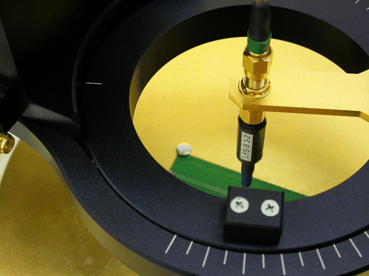
 LFS-B 3-2 scanner probe connected to ICS 105 scanner |
| Frequency response Click image for full view |
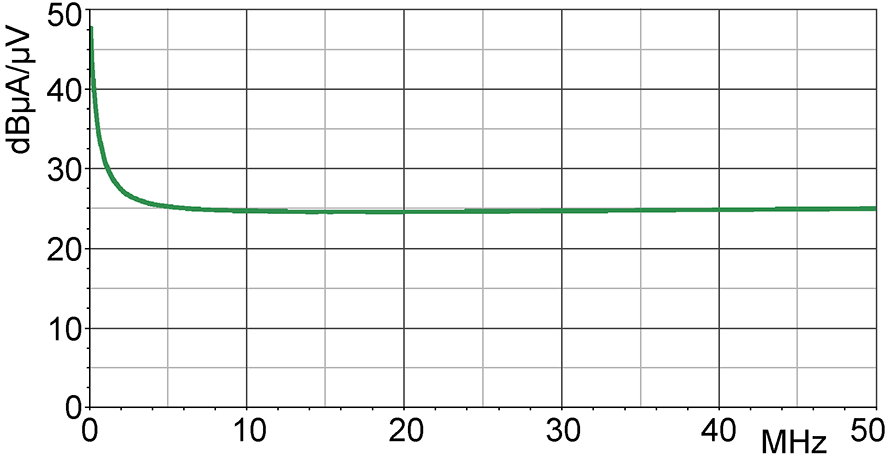
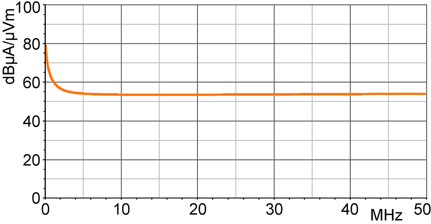
 Frequency response [dBuV] / [dBuA/m] |
| H-field correction curve Click image for full view |
 H-field correction curve [dBuA/m] / [dBuV] |
| Current correction curve Click image for full view |
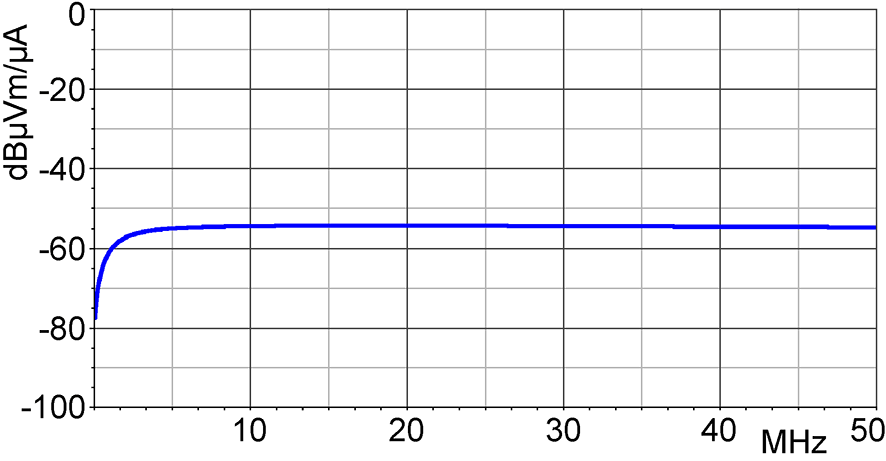
 Current correction curve [dBuA] / [dBuV] |
RFS probe specifications
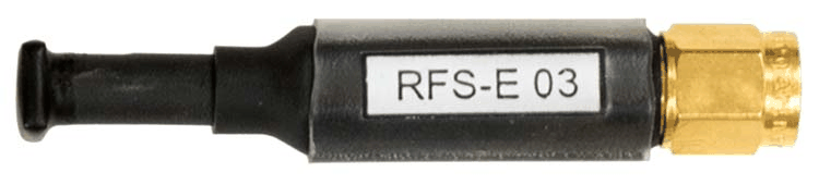
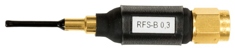
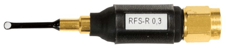
| Specification / view | RFS-R 50 | RFS-R 3-2 | RFS-R 0.3-3 | RFS-B 3-2 | RFS-B 0.3-3 | RFS-E 03 | RFS-E 10 |
|---|---|---|---|---|---|---|---|
| Product picture | |
 |
 |
 |
 |
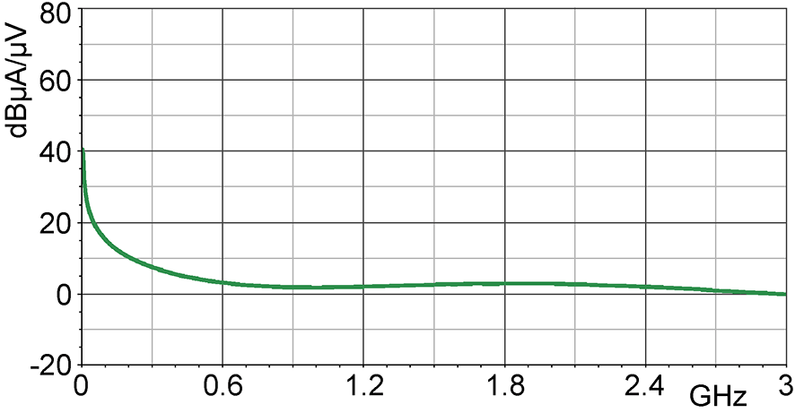 |
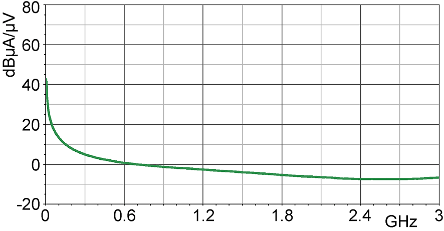 |
| Field type | H-field | H-field | H-field | H-field | H-field | E-field | E-field |
| Included in RFS set | Yes - included | No - separate probe | No - separate probe | Yes - included | No - separate probe | Yes - included | No - separate probe |
| Frequency range | 30 MHz ... 3 GHz | 30 MHz ... 3 GHz | 30 MHz ... 3 GHz | 30 MHz ... 3 GHz | 30 MHz ... 3 GHz | 30 MHz ... 3 GHz | 30 MHz ... 3 GHz |
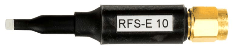
| Probe head dimensions | diameter 10 mm | diameter approx. 3 mm | diameter approx. 2 mm | diameter 2 mm | diameter approx. 2 mm | approx. (4 x 4) mm | approx. (0.5 x 2) mm |
| Connector - output | SMA, male, plug | SMA, male, jack | SMA, male, jack | SMA, male, plug | SMA, male, jack | SMA, male, plug | SMA, male, jack |
| Length | approx. 55 mm | Not specified | Not specified | approx. 55 mm | Not specified | approx. 55 mm | Not specified |
| Resolution | Not specified | approx. 1 mm | < 1 mm | Not specified | < 1 mm | Not specified | approx. 0.2 mm |
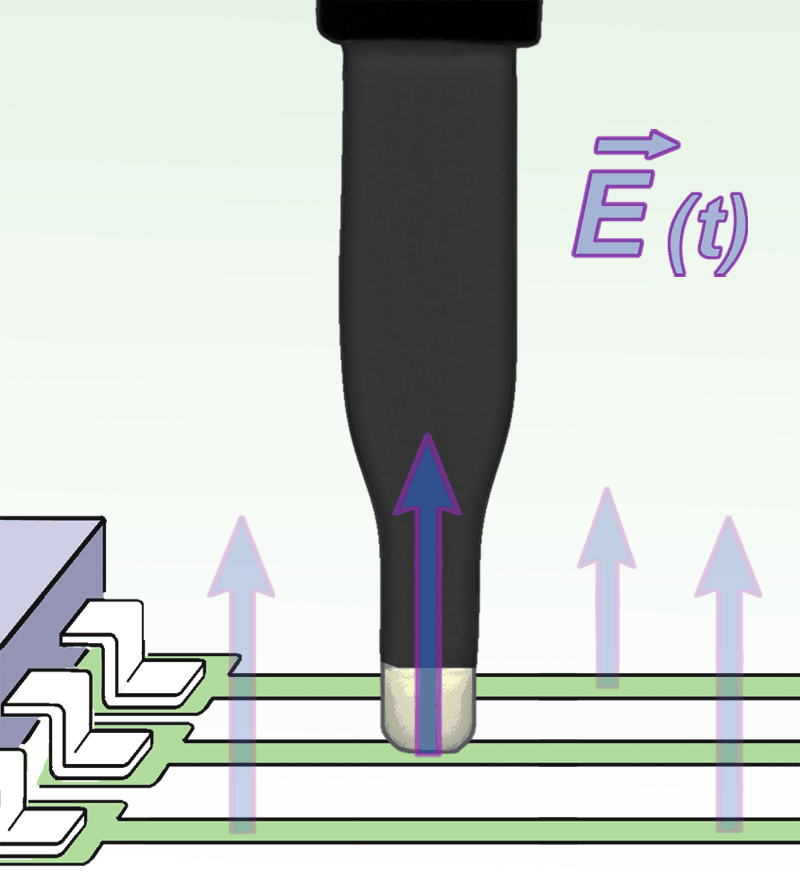
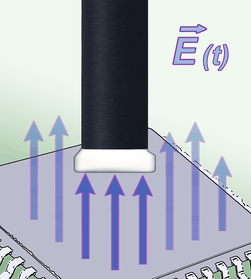
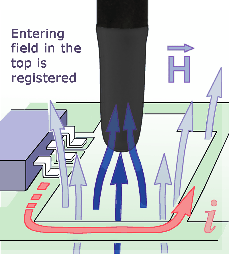
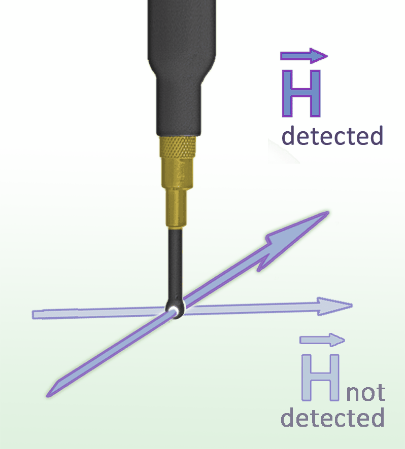
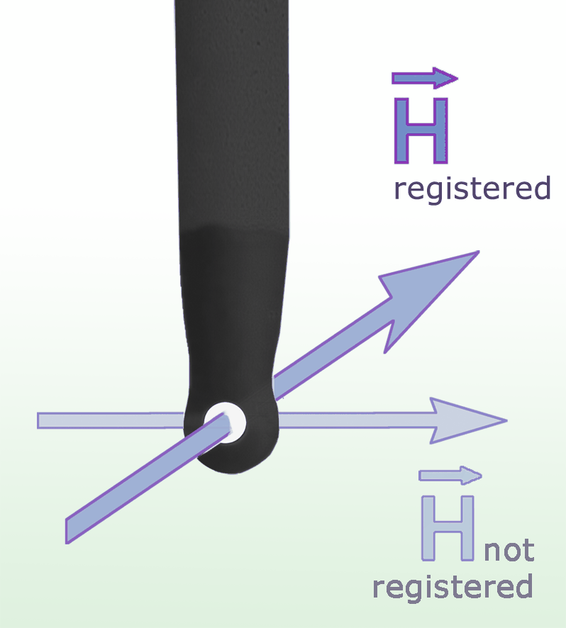
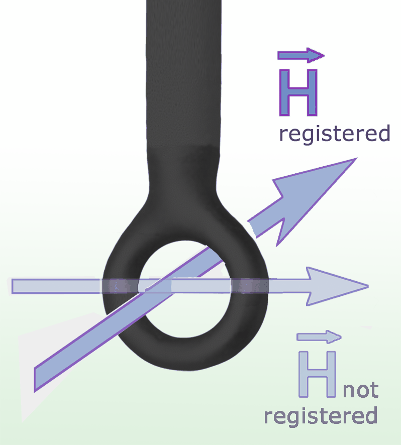
| Use and orientation | H-field; larger-area source search over components and cables, at distances up to approximately 3 cm. Use for overview scans before selecting a finer probe. | H-field; fine mapping near traces, IC pins and packages, decoupling capacitors and EMC components. Align the sensing plane with the field being investigated. | H-field; small head for sub-millimeter localization at small components and hard-to-reach IC pins. | H-field; coil orthogonal to the shaft. Detects field lines normal to the DUT surface; field lines entering laterally are not detected. Close placement gives stronger coupling. | H-field; coil at 90 degrees to the shaft, for very small-scale sensing directly at the DUT. | E-field; approximately 4 x 4 mm electrode underneath the head detects clocked traces, IC pins and small components. | E-field; approximately 0.2 mm electrode width for fine localization at 0.1 mm traces and individual pins on high-pin-count ICs. |
| Sensing orientation Click image for full view |
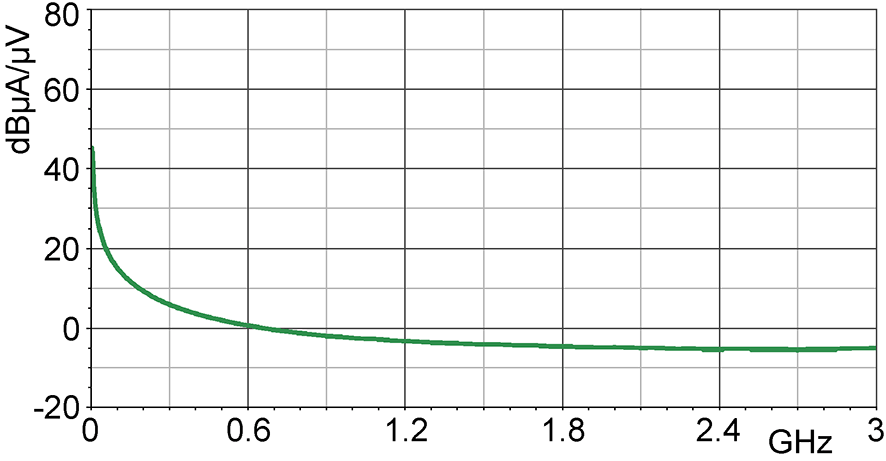 Sensing orientation / measuring principle |
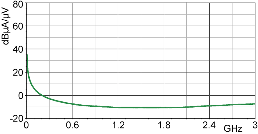 Sensing orientation / measuring principle |
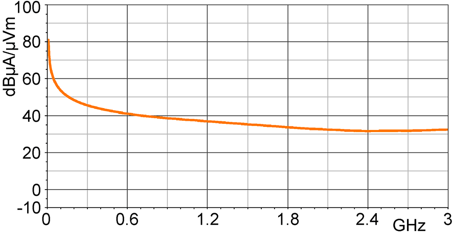 Sensing orientation / measuring principle |
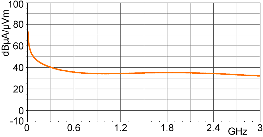 Sensing orientation / measuring principle |
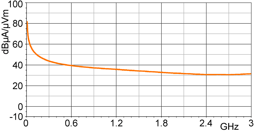 Sensing orientation / measuring principle |
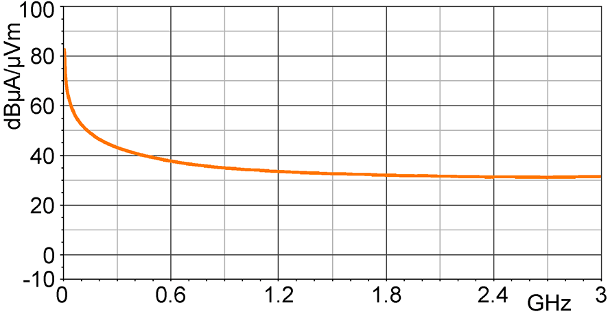 Sensing orientation / measuring principle |
 Sensing orientation / measuring principle |
| Frequency response Click image for full view |
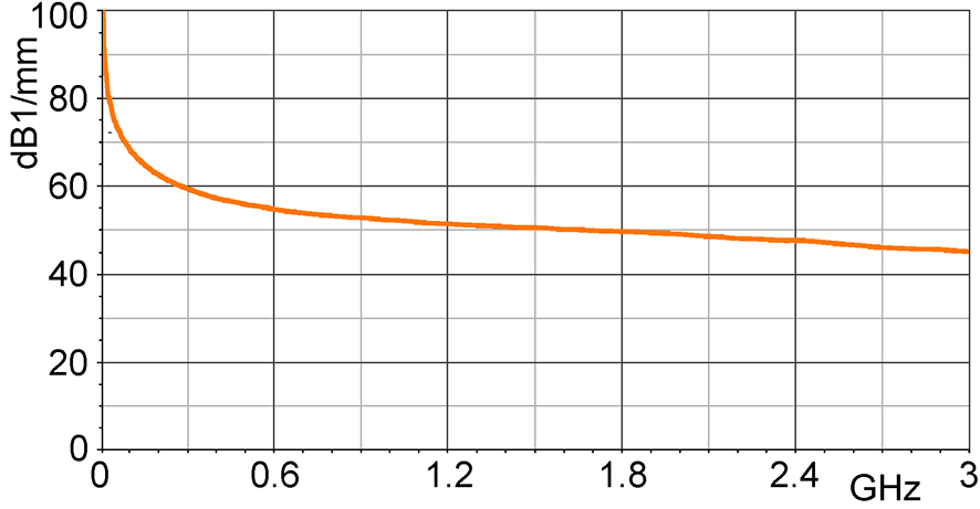
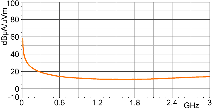
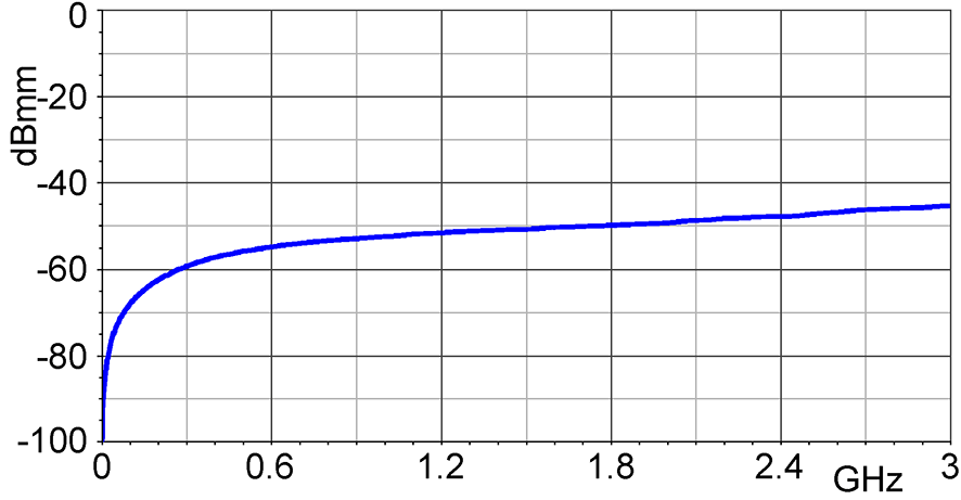 Frequency response |
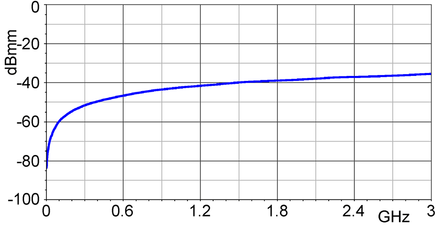 Frequency response [dBuV] / [dBuA/m] |
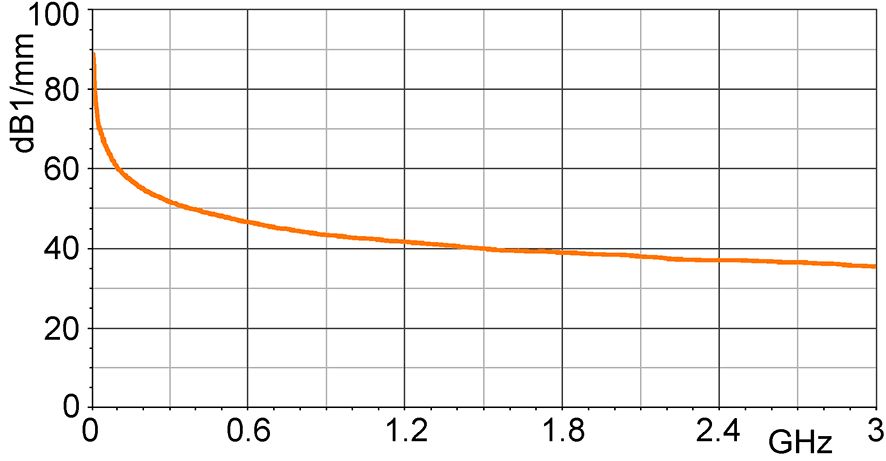
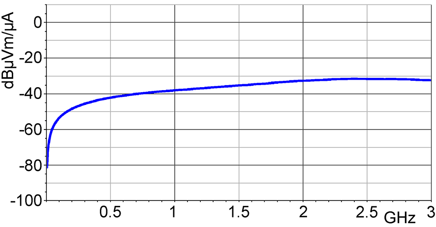 Frequency response [dBuV] / [dBuA/m] |
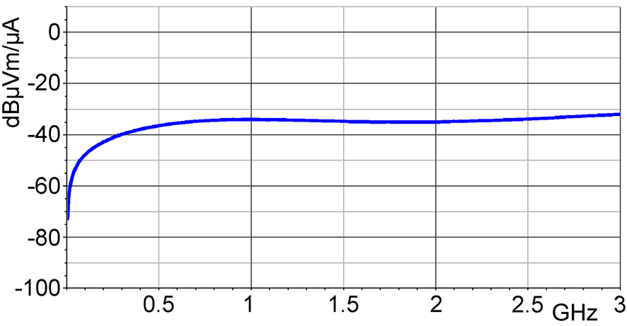 Frequency response |
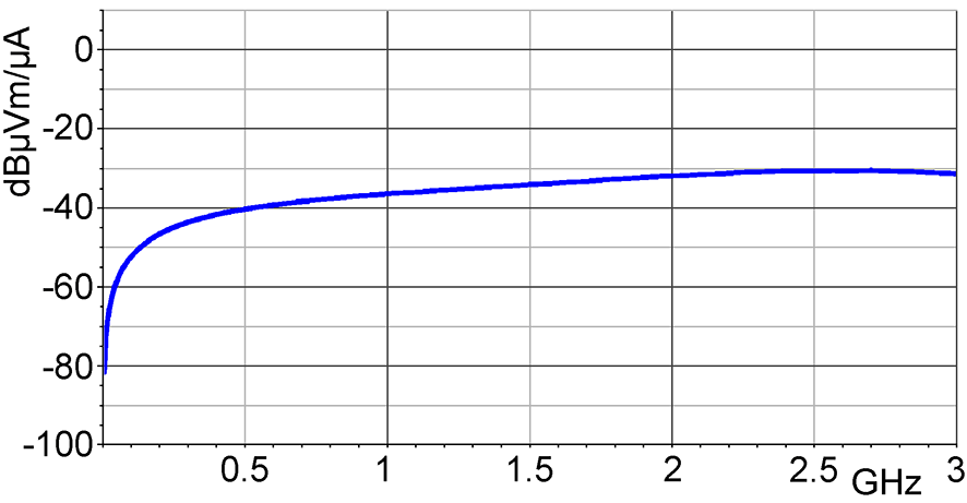 Frequency response [dBuV] / [dBuA/m] |
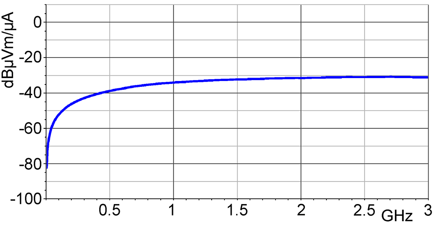 Frequency response |
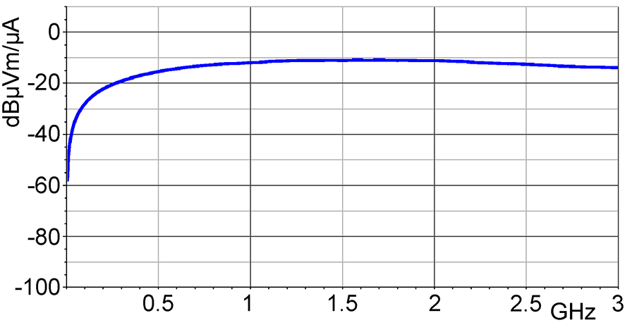 Frequency response [dBuV] / [dBuA/m] |
| H-field correction curve Click image for full view |
 H-field correction curve [dBuA/m] / [dBuV] |
 H-field correction curve [dBuA/m] / [dBuV] |
 H-field correction curve [dBuA/m] / [dBuV] |
 H-field correction curve [dBuA/m] / [dBuV] |
 H-field correction curve [dBuA/m] / [dBuV] |
Not published | Not published |
| Current correction curve Click image for full view |
 Current correction curve [dBuA] / [dBuV] |
 Current correction curve [dBuA] / [dBuV] |
 Current correction curve [dBuA] / [dBuV] |
 Current correction curve [dBuA] / [dBuV] |
 Current correction curve [dBuA] / [dBuV] |
Not published | Not published |
| E-field correction curve Click image for full view |
Not published | Not published | Not published | Not published | Not published | 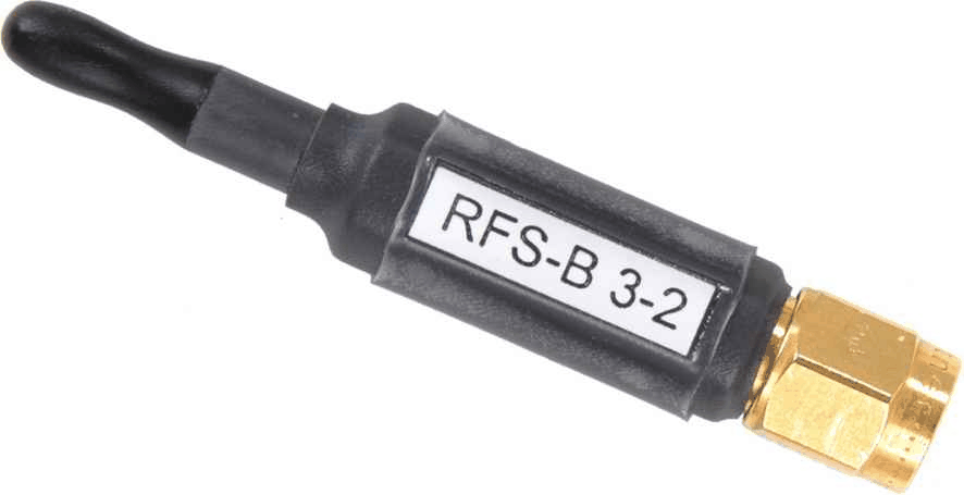 E- field correction curve [dBuV/mm] / [dBuV] |
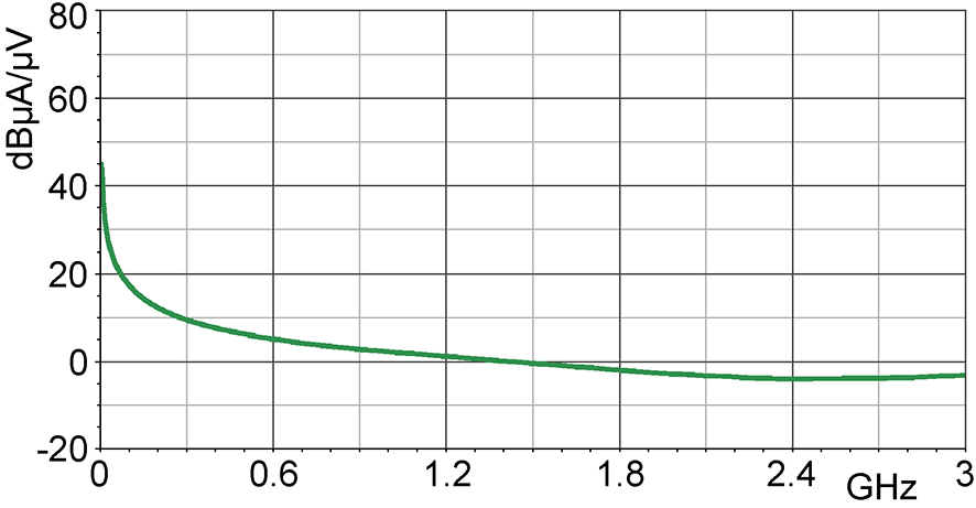
 E- field correction curve [dBuV/mm] / [dBuV] |
XFS probe specifications
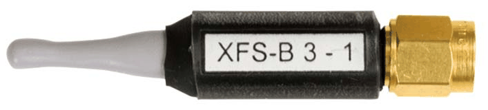
| Specification / view | XFS-R 3-1 | XFS-B 3-1 | XFS-E 10 | XFS-E 09s |
|---|---|---|---|---|
| Product picture | |
 |
 |
 |
| Field type | H-field | H-field | E-field | E-field |
| Frequency range | 30 MHz ... 6 GHz | 30 MHz ... 6 GHz | 30 MHz ... 6 GHz | 30 MHz ... 6 GHz |
| Resolution | approx. 1 mm | approx. 2 mm | approx. 0.2 mm | approx. 0.2 mm |
| Probe head dimensions | diameter approx. 3 mm | diameter approx. 4 mm | approx. (0.5 x 2) mm | approx. (10 x 10) mm |
| Connector - output | SMA, male, jack | SMA, male, jack | SMA, male, jack | SMA, male, jack |
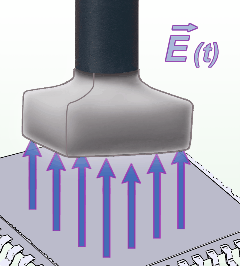
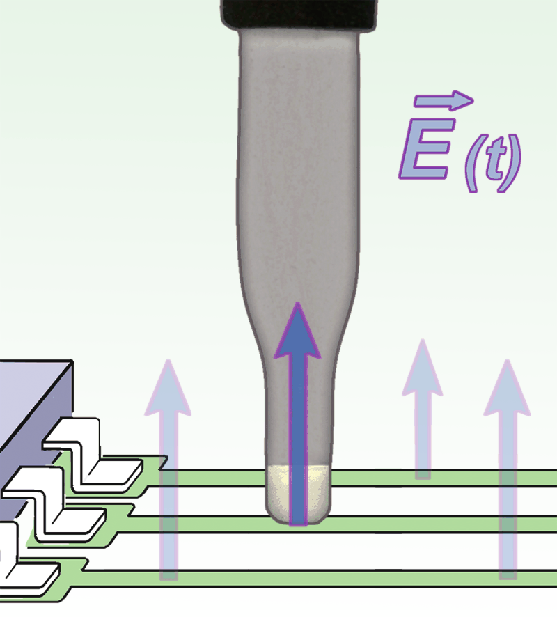
| Use and orientation | H-field; direct high-resolution mapping at traces, IC packages, decoupling capacitors and EMC components, extending coverage to 6 GHz. | H-field; coil orthogonal to the shaft. With the shaft vertical, the sensing coil can be placed directly at the board, including between tall components. | E-field; approximately 0.2 mm electrode width, for 0.1 mm traces and individual IC pins. Position at the structure being measured. | E-field; detects fields above the IC surface. Manufacturer describes measurements from 0.5 to 10 mm above an assembly; choose the spacing for the task. |
| Sensing orientation Click image for full view |
 Sensing orientation / measuring principle |
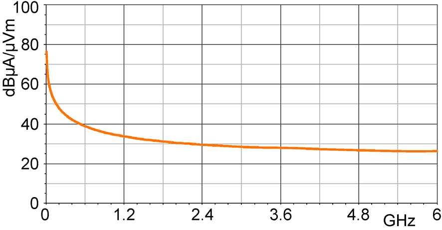 Sensing orientation / measuring principle |
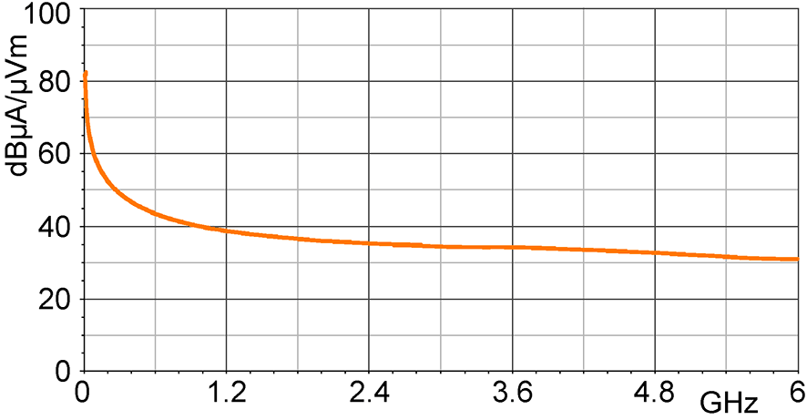 Sensing orientation / measuring principle |
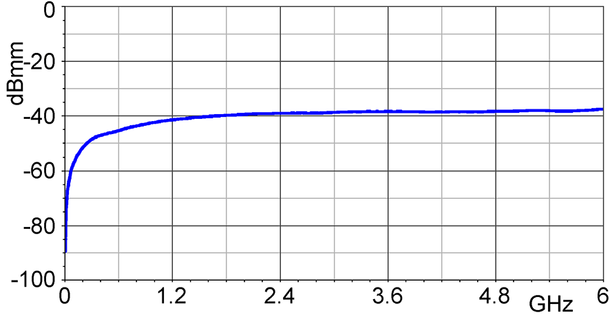 Sensing orientation / measuring principle |
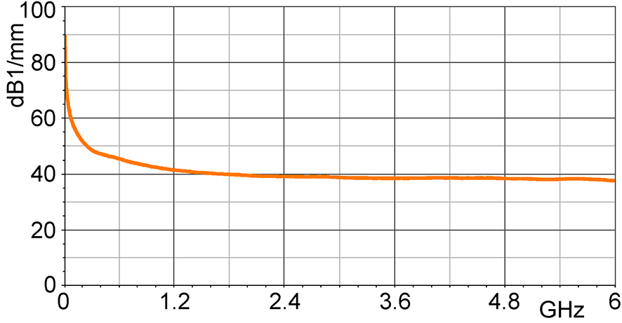
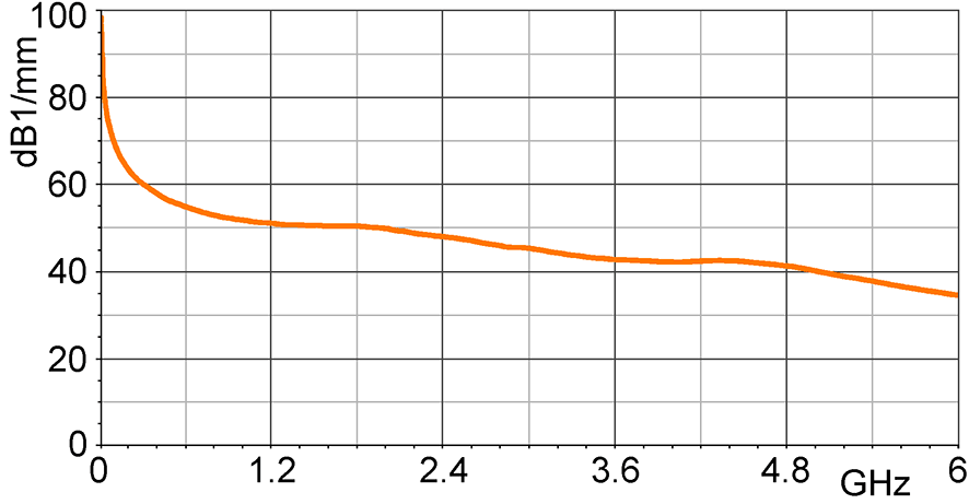
| Frequency response Click image for full view |
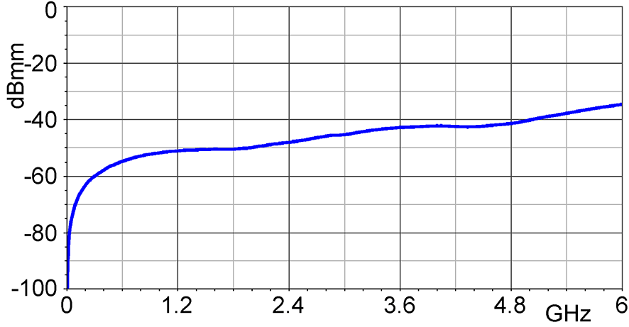 Frequency response [dBuV] / [dBuA/m] |
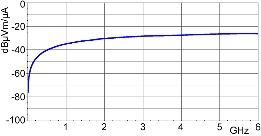 Frequency response [dBuV] / [dBuA/m] |
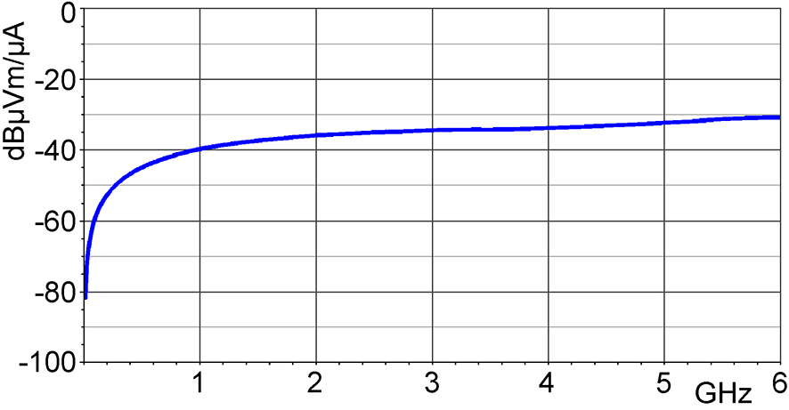 Frequency response [dBuV] / [dBuA/m] |
 Frequency response [dBuV] / [dBuA/m] |
| H-field correction curve Click image for full view |
 H-field correction curve [dBuA/m] / [dBuV] |
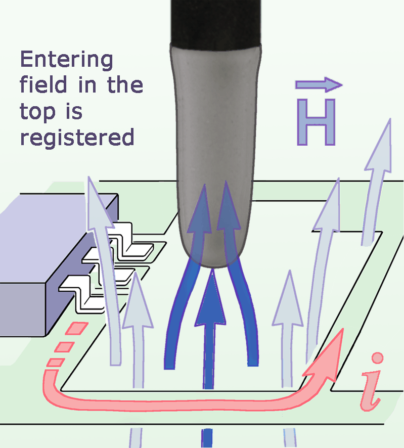 H-field correction curve [dBuA/m] / [dBuV] |
Not published | Not published |
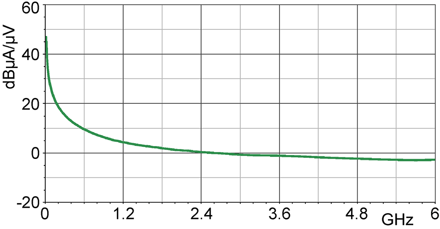
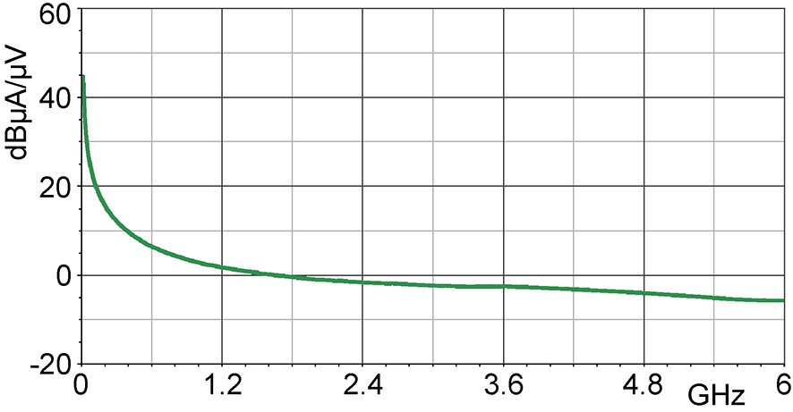
| Current correction curve Click image for full view |
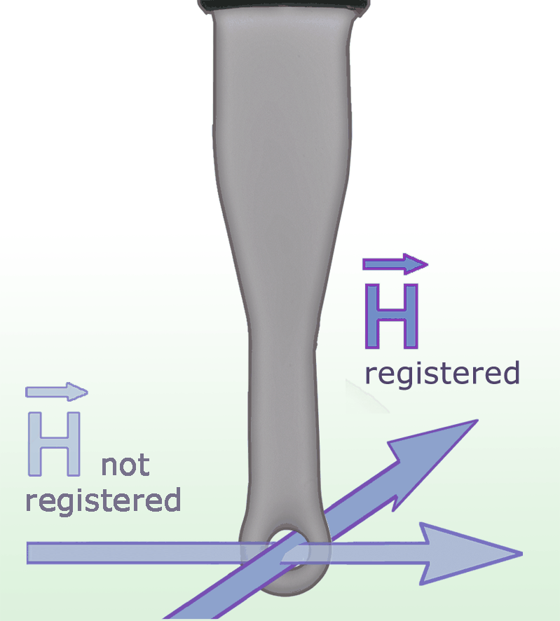 Current correction curve [dBuA] / [dBuV] |
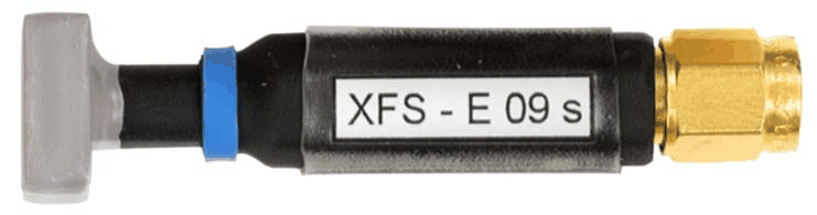 Current correction curve [dBuA] / [dBuV] |
Not published | Not published |
| E-field correction curve Click image for full view |
Not published | Not published | 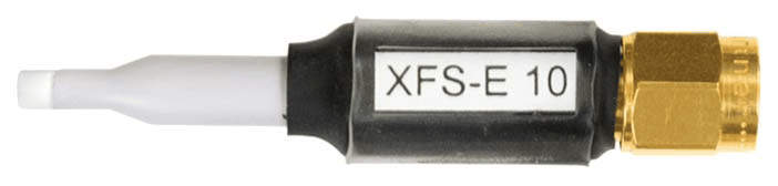 E- field correction curve [dBuV/mm] / [dBuV] |
 E- field correction curve [dBuV/mm] / [dBuV] |
Match the probe to the task
| Task | Starting point | Why |
|---|---|---|
| Switching-current fields below 30 MHz | LFS-B 3 | 100 kHz to 50 MHz coverage. |
| PCB overview and source search | RFS-R 50 | Larger head and approximately 3 cm investigation distance. |
| Fine H-field localization below 3 GHz | RFS-R 0.3-3 / RFS-B 0.3-3 | Published resolution below 1 mm; choose the sensing orientation for the field direction. |
| Fine E-field localization | RFS-E 10 or XFS-E 10 | Approx. 0.2 mm resolution; choose 3 or 6 GHz coverage. |
| PCB scans above 3 GHz | XFS family | 6 GHz upper frequency versus 3 GHz for RFS. |
| Micrometer-scale IC work | ICR near-field microprobes | A separate microprobe family; motion increment and probe spatial resolution must be evaluated together. |
Download spectrum analyzer compatibility and interface guide (PDF). Model, interface, driver-test status, listed firmware and limitations are kept in this separate document. Confirm the software version, firmware and connection before ordering.
Accessories are configured on the scanner pages
Open a scanner page for its pictured full/Basic contents, probe choices and accessories. No separate accessory listings are required.
| Scanner page | Configuration benefit |
|---|---|
| ICS 105 | Choose for a small IC scan area, finer minimum positioning increment and a compact bench footprint. |
| FLS 106 IC | Choose when the DUT or fixture needs a larger area and IC-style angular probe scans are important. |
| FLS 106 PCB | Choose for repeatable X/Y/Z scans over assemblies without the IC model's motorized alpha rotation. |
OTHER PRODUCTS IN THE SAME CATEGORY:

TT 8.0-10t, Turn Table, 8.0m Diameter, 10000kg

PAS 2.0-10kg Pneumatic Antenna Stand
TT 6.0-10t, Turn Table, 6.0m Diameter, 10000kg
TT 5.0-5t, Turn Table, 5.0m Diameter, 5000kg
TT 4.0-4t, Turn Table, 4.0m Diameter, 4000kg
TT 3.0-3t, Turn Table, 3.0m Diameter, 3000kg

MAP 2.5-T Manual Antenna Positioner

EAS 365-15kg Electric Antenna Stand

EAS 1.0/2.0 Electric Antenna Stand

EAS 1.5 10kg Electric Antenna Stand
EAS 1.5 Electric Antenna Stand

BEST 50 - 50 kW Bavarian Engine System Tester

Dynamometer for E-Bike

FR-DYN– 3t-F Dynamometer
F-DYN 4WD – 3t Dynamometer

DYN 4WD - I Dynamometer Integrated into TT 7.5-5t-DYN Turntable

ASP 1.0/1.8-10 kg Pneumatic Antenna Stand
PAS 2.0 Pneumatic Antenna Stand

TAM 4.0-E Boresight Antenna Mast, 4m