Accelerating IEC 61000-4-3 Uniform Field Calibration
Accelerating IEC 61000-4-3 Uniform Field Calibration
Practical methods to reduce calibration time while improving measurement quality
Radiated immunity testing per IEC 61000-4-3 requires verification of field uniformity before exposing an Equipment Under Test (EUT). The standard mandates calibration of a Uniform Field Area (UFA) defined as a 1.5 m × 1.5 m plane subdivided into 16 grid locations. At each point, the electric field must meet specified uniformity criteria over the full test frequency range, commonly 80 MHz to 6 GHz.
While technically straightforward, this calibration is often the most time-consuming step in radiated immunity testing. For broadband chambers, a traditional single-probe calibration can take many days, and if the results do not meet requirements, rescans are needed, reducing chamber availability and increasing operating costs.
By combining faster instrumentation, automation, and multi-probe strategies, calibration time can be reduced by factors of 2x, 4×, to 16× All while increasing compliance and measurement integrity.
This article outlines practical approaches from conventional methods through high-throughput solutions, enabling laboratories to select the optimal balance of cost, complexity, and speed.
Standard Method: Single-Probe Sequential Calibration
Procedure
- Configure the chamber with the transmitting antenna, amplifier chain, forward power measurement, and no EUT present.
- Place one calibrated isotropic field probe at grid location #1.
- Sweep the full frequency range.
- At each frequency, adjust forward power until the target field strength is reached and log the required power.
- Move the probe to the next grid position.
- Repeat until all 16 locations are measured for each polarization.
Limitations
This method requires:
- 16 complete frequency sweeps per polarization
- Manual repositioning at each grid point
- Operator attendance for many hours
- Significant dwell time for probe settling
For wideband calibrations, total acquisition time frequently exceeds 12–16 hours.
The bottleneck is not RF power generation, but measurement and repositioning time.
Step 1 – Faster Measurements with High-Speed Probes
Concept
Many traditional field probes require settling or averaging time at each frequency step to stabilize their reading. This dwell time significantly increases sweep duration.
A high-speed field probe with rapid detector response and fast digital sampling:
- Reacts quickly to field changes
- Requires minimal settling time
- Reduces per-frequency measurement time
Supporting Requirement
If the probe measures quickly, the forward power feedback loop must also be fast. Therefore:
- Use a high-speed power meter
- Minimize control-loop latency in the test software
Result
Reducing measurement dwell from, for example, 2–4 s to 50–100 ms per step can cut sweep time by 1000x+, even before addressing probe movement.
Benefit
- Faster calibration, reduce total 16-point calibration to much less than 1 day
- Improved statistical repeatability (less drift during measurement)
- Better overall chamber utilization
Equipment: LUMILOOP LSProbe 1.2 Variant E + LSPM 1.0 Power Meter

LSProbe CI-250 with LSPM 1.0 in 19″ Rack
or

CI-250+ with LSPM 1.0 in 19″ Rack
Step 2 – Automating Probe Positioning
Concept
Manual movement of the probe between 16 grid locations adds:
- Operator labor
- Inconsistent placement
- Idle time between sweeps
Automated positioning removes these inefficiencies.
Procedure
- Mount probe on a motorized X–Y positioner.
- Run sweep at location #1.
- Automatically move to location #2.
- Repeat until all 16 locations are complete.
Advantages
- Fully unattended operation
- Repeatable positioning
- Overnight calibration possible
- Reduced operator time
Result
Time savings from automation typically reduce total calibration time by 30–50% while improving consistency.
Equipment: FPP2.3/1.5 Field Probe Positioner + FCU3.0S USB Controller


Step 3 – Parallel Measurements with Multiple Probes
The next improvement is reducing the number of required sweeps by measuring multiple points simultaneously.
Two Probes
- Measure 2 locations per sweep
- Time cut in half
Equipment: LUMILOOP 2x LSProbe 1.2 Variant E + LSPM 1.0 Power Meter

2x LSProbe CI-250 with LSPM 1.0 in 19″ Rack
or
![]()

2x LSProbe CI-250+ with LSPM 1.0 in 19″ Rack
Four Probes
- Measure 4 locations per sweep
- Time reduced to ¼
Equipment: LUMILOOP 4x LSProbe 1.2 Variant E + LSPM 1.0 Power Meter
FPP2.3/1.5 M Field Probe Positioner + FCU3.0S

4xLSProbe CI-250 with LSPM 1.0 in 19″ Rack
or

1x CI-250+, 3xLSProbe CI-250 with LSPM 1.0 in 19″ Rack


FPP2.3/1.5 M Field Probe Positioner + FCU3.0S
Sixteen Probes
- Measure all points simultaneously
- Single sweep only
- Fastest possible solution


2 kits of 8x LSProbe 1.2, Variant E Part No. 3110
Trade-Off
While 16 probes provide maximum throughput, the cost of purchasing and maintaining 16 calibrated broadband probes can be substantial.
Practical High-Efficiency Solution – Four Probes with Automatic Positioner
For many laboratories, the optimal balance between performance and cost is a 4-probe array with automated repositioning.
Concept
- Four probes mounted to a precision frame
- Positioner moves the array to four locations
- Four sweeps total → covers all 16 grid points
Procedure
- Place the probe array in the first quadrant (4 points).
- Run a full frequency sweep.
- Move the array to the second quadrant.
- Repeat for all four positions.
- Stitch datasets into full 16-point calibration matrix.
Performance Comparison
| Method | Sweeps Required | Relative Time* |
| Standard Probe | 16 | 12-16 hr |
| 1-LSProbe & LSPM | 16 | 100% (~4 hr) |
| 1-LSProbe & LSPM + Positioner | 16 | 75% (~3hr) |
| 2-LSProbe & LSPM + Positioner | 8 | 38% (~2hr) |
| 4-LSProbes & LSPM + positioner | 4 | 19% (~1hr) |
| 16-LSProbes & LSPM + 4-Probe Stands | 1 | 5% (minutes) |
* Test time has many factors that are not covered in this article, such as amplifier and antenna bands, where manual changes in setup may be required, adding additional time. The table illustrates how the test setup improvements affect time.
Advantages
- 81% reduction in test time
- Far lower cost than 16 probes
- Automated, unattended operation
- Excellent repeatability
- Flexible for alternate grid sizes or chamber mapping
This approach delivers most of the speed benefit of a 16-probe system at a fraction of the capital cost.
Complete Optimization Strategy
Maximum efficiency is achieved when combining all improvements:
Recommended Configuration
- Fast broadband field probes
- Fast power meter/feedback loop
- Automated positioner
- Multi-probe array (4 or more)
Combined Effect
When implemented together:
- Faster per-frequency acquisition
- Reduced number of sweeps
- No manual intervention
- Consistent positioning
Calibration that previously required a full day can often be completed in 1–3 hours.
Operational Benefits
Reducing calibration time directly improves:
- Chamber availability
- Throughput
- Labor efficiency
- Cost per test
- Ability to validate multiple setups quickly
- Flexibility to characterize different chamber regions
For facilities with multiple chambers or frequent recalibrations, time savings translate directly into higher revenue capacity.
Conclusion
IEC 61000-4-3 uniform field calibration does not have to be a bottleneck.
By progressively implementing:
- High-speed probes
- Fast power measurement
- Automated movement
- Parallel multi-probe acquisition
Laboratories can dramatically shorten calibration time while improving repeatability and data quality.
For most organizations, a 4-probe automated positioner system offers the best balance of cost and performance, while a 16-probe array provides ultimate throughput for high-volume environments.
Absolute EMC provides scalable solutions—from single-probe automation to full multi-probe systems—allowing each lab to select the configuration that matches its throughput and budget requirements.